BIDS stats model
This file allows you to specify the GLM to run and which contrasts to compute.
It follows BIDS statistical model.
This type of JSON file is a bit more complicated than the usual JSON files, you might be acquainted with in BIDS. So make sure you have a read through the JSON 101 page.
Then have a look at the walkthrough that explains how to build a simple model.
Validate your model
In Visual Studio Code
You can add those lines to the .vscode/settings.json of your project to help
you validate BIDS stats models as you write them.
{
  "json.schemas": [
    {
      "fileMatch": [
        "model-*_smdl.json"
      ],
      "url": "https://bids-standard.github.io/stats-models/BIDSStatsModel.json"
    }
  ],
  "esbonio.sphinx.confDir": ""
}
In the browser
Otherwise you can use the online validator and copy paste your model in it.
Using the BIDS stats model python package
Requires python and pip.
From within the bidspm folder open a terminal and install the bidspm package.
pip install .
Then you can validate your model with the following command.
validate_model path_to_your_model_json
Loading and interacting with a BIDS stats model
You can use the BidsModel class to create a bids model instance and interact
with. This class inherits from bids-matlab bids.Model class.
- class BidsModel
- Property Summary
- SPM
content of SPM.mat
- Method Summary
- getHRFderivatives(varargin)
returns the HRF derivatives of a node of a BIDS statistical model
- getInclusiveMaskThreshold(varargin)
returns the threshold for inclusive masking of subject level GLM node of a BIDS statistical model
- getModelMask(varargin)
returns the mask of a node of a BIDS statistical model
- getSerialCorrelationCorrection(varargin)
returns the Serial Correlation Correction of a node of a BIDS statistical model
- validateConstrasts()
validate all contrasts spec in the model
There are also extra functions to interact with those models.
src.bids_model.getContrastsList()src.bids_model.getDummyContrastsList()
bidspm implementation of the BIDS stats model
bidspm only implements a subset of what is currently theoretically possible with the BIDS stats model.
For example, at the subject level the bidspm can only access variables, that are
in the events.tsv in that raw dataset or in the regressors.tsv or
timeseries.tsv generated by the preprocessing pipeline.
At the group level, it is only possible to access some variables from the
participants.tsv file.
Transformation
The Transformations object allows you to define what you want to do to some
variables, before you put them in the design matrix.
Currently bidspm can only transform variables contained in events.tsv files.
It uses bids-matlab transformers to run those transformations. Please see this bids-matlab documentation to know how to use them and call them in your JSON.
You can find a list of the available variables transformations in the bids matlab doc and on the variable-transforms repository
The advantage of these bids-matlab transformers is that they allow you to directly test them on tsv files to quickly see what outcome a series of transformers will produce.
Below is an example on how to subtract 3 seconds from the event onsets of the
conditions motion listed in the trial_type columns of the events.tsv file,
and put the output in a variable called motion.
"Transformations": {
    "Transformer": "bidspm",
    "Instructions": [
        {
            "Name": "Subtract",
            "Input": [
              "onset"
            ],
            "Query": "trial_type==motion",
            "Value": 3,
            "Output": [
                "motion"
            ]
        }
    ]
}
At the subject level, bidspm can only access apply transformation on the content
events.tsv.
You can find demo of how to design the transformers for your analysis
in the demos/transformers folder and
also in demos/ds003717/code/04_transformation.m.
HRF
For a given Node, Model.X defines the variables that have to be put in the
design matrix.
Here trans_? means any of the translation parameters (in this case trans_x,
trans_y, trans_z) from the realignment that are stored in _confounds.tsv
files.
Similarly *outlier* means that ANY “scrubbing” regressors containing the word
outlier created by fMRIprep or bidspm to detect motion outlier or potential
dummy scans will be included.
"Model": {
    "Type": "glm",
    "X": [
        "motion",
        "static",
        "trans_?",
        "rot_?",
        "*outlier*"
    ],
    "HRF": {
        "Variables": [
            "motion",
            "static"
        ],
        "Model": "spm"
    }
}
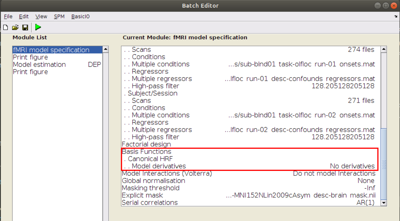
HRF specifies:
which variables of
Xhave to be convolvedwhat HRF model to use to do so.
You can choose from:
"spm""spm + derivative""spm + derivative + dispersion"
Not yet implemented:
"fir"
Software
By default, bidspm will use SPM’s FAST model for the SerialCorrelation model.
It will also use a value of 0.8 for the InclusiveMaskingThreshold
to define the implicit inclusive mask
that is used by SPM to determine in which voxels the GLM will be estimated
(the value is taken fromdefaults.mask.thresh from SPM’s defaults).
This corresponds to explicitly setting the following fields in the Model.Software.SPM
object of a node in the BIDS stats model.
{
  "Nodes": [
    {
      "Level": "Run",
      "Name": "run_level",
      "Model": {
        "X": ["trial_type.listening"],
        "HRF": {
          "Variables": ["trial_type.listening"],
          "Model": "spm"
        },
        "Type": "glm",
        "Software": {
          "SPM": {
            "SerialCorrelation": "FAST",
            "InclusiveMaskingThreshold": 0.8
          }
        }
      }
    }
  ]
}
These values will explicitly be added to your your default BIDS stats model if you use bidspm ‘default_model’ action.
bidspm(bids_dir, output_dir, 'dataset', ...
        'action', 'default_model')
Note that if you wanted to use the AR(1) model for the serial correlation
and to include all voxels in the implicit mask,
you would have to set the following:
{
  "Nodes": [
    {
      "Level": "Run",
      "Name": "run_level",
      "Model": {
        "X": ["trial_type.listening"],
        "HRF": {
          "Variables": ["trial_type.listening"],
          "Model": "spm"
        },
        "Type": "glm",
        "Software": {
          "SPM": {
            "SerialCorrelation": "AR(1)",
            "InclusiveMaskingThreshold": "-Inf"
          }
        }
      }
    }
  ]
}

Corresponding options in SPM batch
Results
It is possible to specify the results you want to view directly the
Model.Software object of any Nodes in the BIDS stats model.
See the help section of the bidsResults function for more detail, but here is
an example how you could specify it in a JSON.
"Model": {
    "Software": {
        "bidspm": {
          "Results": [
              {
                "name": [
                    "contrast_name", "other_contrast_name"
                ],
                "p": 0.05,
                "MC": "FWE",
                "png": true,
                "binary": true,
                "nidm": true,
                "montage": {
                    "do": true,
                    "slices": [
                    -4,
                    0,
                    4,
                    8,
                    16
                    ],
                    "background": {
                    "suffix": "T1w",
                    "desc": "preproc",
                    "modality": "anat"
                    }
                }
              },
              {
                "Description": "Note that you can specify multiple results objects, each with different parameters.",
                "name": [
                    "yes_another_contrast_name"
                ],
                "p": 0.01,
                "k": 10,
                "MC": "none",
                "csv": true,
                "atlas": "AAL"
              }
          ]
        }
    }
}
Contrasts
Run level
To stay close to the way most SPM users are familiar with, all runs are analyzed in one single GLM.
Contrasts are the run level that are either specified using DummyContrasts or
Contrasts will be computed and will have the run number appended to their name
in the SPM gui as shown in Contrast for run 1 and Contrast for run 2.
{
  "Level": "Run",
  "Name": "run_level",
  "X": [
    "olfid_eucalyptus_left",
    "olfid_eucalyptus_right",
    "olfid_almond_left",
    "olfid_almond_right",
    "olfloc_eucalyptus_left",
    "olfloc_eucalyptus_right",
    "olfloc_almond_left",
    "olfloc_almond_right",
    "resp_03",
    "resp_12",
    1
  ],
  "DummyContrasts": {
    "Contrasts": [
      "olfid_eucalyptus_left",
      "olfid_eucalyptus_right",
      "olfid_almond_left",
      "olfid_almond_right",
      "olfloc_eucalyptus_left",
      "olfloc_eucalyptus_right",
      "olfloc_almond_left",
      "olfloc_almond_right"
    ],
    "Test": "t"
  },
  "Contrasts": [
    {
      "Name": "olfid",
      "ConditionList": [
        "olfid_eucalyptus_left",
        "olfid_eucalyptus_right",
        "olfid_almond_left",
        "olfid_almond_right"
      ],
      "Weights": [
        1,
        1,
        1,
        1
      ],
      "Test": "t"
    }
  ]
}
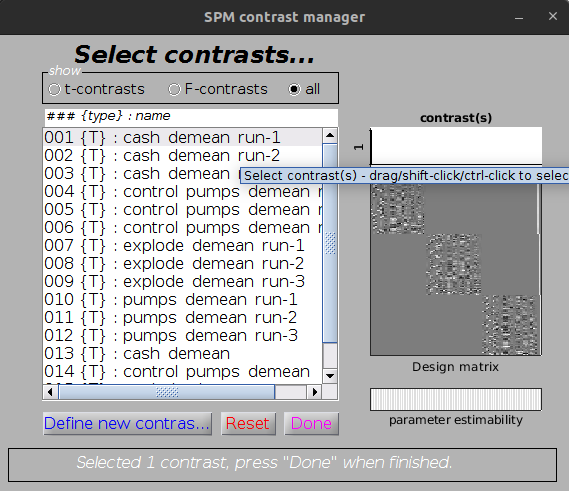
Contrast for run 1

Contrast for run 2
Subject level
At the moment the only type of model supported at the run level is averaging of run level contrasts.
{
  "Level": "Subject",
  "Name": "subject_level",
  "Description": "Only averaging at the subject level is supported for now.",
  "GroupBy": [
    "contrast",
    "subject"
  ],
  "Model": {
    "X": [
      1
    ],
    "Type": "glm"
  },
  "DummyContrasts": {
    "Test": "t"
  }
}

Subject level contrast averaging beta of run 1 and 2
Dataset level
At the moment only, the only type of models that are supported are:
one sample t-test: averaging across all subjects
{
  "Level": "Dataset",
  "Name": "dataset_level",
  "GroupBy": [
    "contrast"
  ],
  "Model": {
    "X": [
      1
    ],
    "Type": "glm"
  },
  "DummyContrasts": {
    "Test": "t"
  }
}
one sample t-test: averaging across all subjects of a specific group
{
  "Level": "Dataset",
  "Name": "within_group",
  "Description": "one sample t-test for each group",
  "GroupBy": [
    "contrast",
    "Group"
  ],
  "Model": {
    "Type": "glm",
    "X": [
      1
    ]
  },
  "DummyContrasts": {
    "Test": "t"
  }
}
2 samples t-test: comparing 2 groups
At the moment this can only be based on how participants are allocated to a
group based on a group or Group column in the participants.tsv of in the
raw dataset.
{
  "Level": "Dataset",
  "Name": "between_groups",
  "Description": "2 sample t-test between groups",
  "GroupBy": [
    "contrast"
  ],
  "Model": {
    "Type": "glm",
    "X": [
      1,
      "group"
    ]
  },
  "Contrasts": [
    {
      "Name": "blind_gt_control",
      "ConditionList": [
        "Group.blind",
        "Group.control"
      ],
      "Weights": [
        1,
        -1
      ],
      "Test": "t"
    }
  ]
}
Method section
It is possible to write a draft of method section based on a BIDS statistical model.
opt.model.file = fullfile(pwd, ...
                          'models', ...
                          'model-faceRepetition_smdl.json');
opt.fwhm.contrast = 0;
opt = checkOptions(opt);

opt.designType = 'block';

outputFile = boilerplate(opt, ...
                        'outputPath', pwd, ...
                        'pipelineType', 'stats');
## fMRI statistical analysis

The fMRI data were analysed with bidspm (v2.2.0; https://github.com/cpp-lln-lab/bidspm; DOI: https://doi.org/10.5281/zenodo.3554331)
using statistical parametric mapping
(SPM12 - 7771; Wellcome Center for Neuroimaging, London, UK;
https://www.fil.ion.ucl.ac.uk/spm; RRID:SCR_007037)
using MATLAB 9.4.0.813654 (R2018a)
on a unix computer (Linux version 5.15.0-53-generic (build@lcy02-amd64-047) (gcc (Ubuntu 11.2.0-19ubuntu1) 11.2.0, GNU ld (GNU Binutils for Ubuntu) 2.38) #59-Ubuntu SMP Mon Oct 17 18:53:30 UTC 2022
).

The input data were the preprocessed BOLD images in IXI549Space space for the task " facerepetition ".

### Run / subject level analysis

At the subject level, we performed a mass univariate analysis with a linear
regression at each voxel of the brain, using generalized least squares with a
global  AR(1)  model to account for temporal auto-correlation
 and a drift fit with discrete cosine transform basis ( 128 seconds cut-off).

Image intensity scaling was done run-wide before statistical modeling such that
the mean image would have a mean intracerebral intensity of 100.

We modeled the fMRI experiment in a  event  design with regressors
entered into the run-specific design matrix. The onsets
were convolved with SPM canonical hemodynamic response function (HRF)
 and its temporal and dispersion derivatives for the conditions:
  - `famous_1`,
 - `famous_2`,
 - `unfamiliar_1`,
 - `unfamiliar_2`,
 .

 Nuisance covariates included:

 - `trans_?`,
 - `rot_?`,

to account for residual motion artefacts,
 .


 ## References

This method section was automatically generated using bidspm
(v2.2.0; https://github.com/cpp-lln-lab/bidspm; DOI: https://doi.org/10.5281/zenodo.3554331)
and octache (https://github.com/Remi-Gau/Octache).
Parametric modulation
Those are not yet fully implemented but there is an example of how to get started in the face repetition demo folder.
{
  "Name": "parametric modulation",
  "BIDSModelVersion": "1.0.0",
  "Description": "model for face repetition",
  "Input": {
    "task": [
      "facerepetition"
    ],
    "space": [
      "IXI549Space"
    ]
  },
  "Nodes": [
    {
      "Level": "Run",
      "Name": "parametric",
      "GroupBy": [
        "run",
        "subject"
      ],
      "Transformations": {
        "Description": "merge the familiarity and repetition column to create the trial type column",
        "Transformer": "bidspm",
        "Instructions": [
          {
            "Name": "Concatenate",
            "Input": [
              "face_type",
              "repetition_type"
            ],
            "Output": "trial_type"
          }
        ]
      },
      "Model": {
        "X": [
          "trial_type.famous_first_show",
          "trial_type.famous_delayed_repeat",
          "trial_type.unfamiliar_first_show",
          "trial_type.unfamiliar_delayed_repeat",
          "trans_?",
          "rot_?"
        ],
        "HRF": {
          "Variables": [
            "trial_type.famous_first_show",
            "trial_type.famous_delayed_repeat",
            "trial_type.unfamiliar_first_show",
            "trial_type.unfamiliar_delayed_repeat"
          ],
          "Model": "spm"
        },
        "Type": "glm",
        "Options": {
          "HighPassFilterCutoffHz": 0.0078,
          "Mask": {
            "suffix": [
              "mask"
            ],
            "desc": [
              "brain"
            ]
          }
        },
        "Software": {
          "SPM": {
            "SerialCorrelation": "AR(1)",
            "ParametricModulations": [
              {
                "Name": "lag mod",
                "Conditions": [
                  "trial_type.famous_delayed_repeat",
                  "trial_type.unfamiliar_delayed_repeat"
                ],
                "Values": [
                  "lag"
                ],
                "PolynomialExpansion": 2
              }
            ]
          }
        }
      },
      "DummyContrasts": {
        "Test": "t",
        "Contrasts": [
          "trial_type.famous_first_show",
          "trial_type.famous_delayed_repeat",
          "trial_type.unfamiliar_first_show",
          "trial_type.unfamiliar_delayed_repeat"
        ]
      },
      "Contrasts": [
        {
          "Name": "faces_gt_baseline",
          "ConditionList": [
            "trial_type.famous_first_show",
            "trial_type.famous_delayed_repeat",
            "trial_type.unfamiliar_first_show",
            "trial_type.unfamiliar_delayed_repeat"
          ],
          "Weights": [
            1,
            1,
            1,
            1
          ],
          "Test": "t"
        },
        {
          "Name": "faces_lt_baseline",
          "ConditionList": [
            "trial_type.famous_first_show",
            "trial_type.famous_delayed_repeat",
            "trial_type.unfamiliar_first_show",
            "trial_type.unfamiliar_delayed_repeat"
          ],
          "Weights": [
            -1,
            -1,
            -1,
            -1
          ],
          "Test": "t"
        }
      ]
    }
  ]
}
See the help section of convertOnsetTsvToMat for more information.
Examples
There are several examples of models in the model zoo along with links to their datasets.
Several of the demos have their own model and you can find several “dummy” models (without corresponding data) used for testing in this folder.
An example of JSON file could look something like that:
{
  "Name": "vislocalizer",
  "BIDSModelVersion": "1.0.0",
  "Description": "contrasts for the visual localizer",
  "Input": {
    "task": [
      "vislocalizer"
    ],
    "space": [
      "IXI549Space"
    ]
  },
  "Nodes": [
    {
      "Level": "Run",
      "Name": "run_level",
      "GroupBy": [
        "run",
        "subject"
      ],
      "Model": {
        "Type": "glm",
        "X": [
          "trial_type.VisMot",
          "trial_type.VisStat",
          "trial_type.missing_condition",
          "trans_?",
          "rot_?"
        ],
        "HRF": {
          "Variables": [
            "trial_type.VisMot",
            "trial_type.VisStat"
          ],
          "Model": "spm+derivative"
        },
        "Options": {
          "HighPassFilterCutoffHz": 0.008,
          "Mask": {
            "desc": [
              "brain"
            ],
            "suffix": [
              "mask"
            ]
          }
        },
        "Software": {
          "SPM": {
            "InclusiveMaskingThreshold": 0.8,
            "SerialCorrelation": "FAST"
          },
          "bidspm": {
            "Results": [
              {
                "name": [
                  "VisMot_&_VisStat"
                ],
                "p": 0.001,
                "MC": "none"
              },
              {
                "name": [
                  "VisStat",
                  "VisMot"
                ],
                "k": 10
              }
            ]
          }
        }
      },
      "DummyContrasts": {
        "Test": "t",
        "Contrasts": [
          "trial_type.VisMot",
          "trial_type.VisStat"
        ]
      },
      "Contrasts": [
        {
          "Name": "VisMot_&_VisStat",
          "ConditionList": [
            "trial_type.VisMot",
            "trial_type.VisStat"
          ],
          "Weights": [
            1,
            1
          ],
          "Test": "t"
        },
        {
          "Name": "VisMot_&_VisStat_lt_baseline",
          "ConditionList": [
            "trial_type.VisMot",
            "trial_type.VisStat"
          ],
          "Weights": [
            -1,
            -1
          ],
          "Test": "t"
        }
      ]
    },
    {
      "Level": "Subject",
      "Name": "subject_level",
      "GroupBy": [
        "contrast",
        "subject"
      ],
      "Model": {
        "Type": "glm",
        "X": [
          1
        ],
        "Options": {
          "Mask": {
            "desc": [
              "brain"
            ],
            "suffix": [
              "mask"
            ]
          }
        },
        "Software": {
          "bidspm": {
            "Results": [
              {
                "name": [
                  "VisMot_&_VisStat"
                ],
                "p": 0.001,
                "MC": "FDR"
              }
            ]
          }
        }
      },
      "DummyContrasts": {
        "Test": "t"
      }
    },
    {
      "Level": "Dataset",
      "Name": "dataset_level",
      "GroupBy": [
        "contrast"
      ],
      "Model": {
        "Type": "glm",
        "X": [
          1
        ],
        "Options": {
          "Mask": {
            "desc": [
              "brain"
            ],
            "suffix": [
              "mask"
            ]
          }
        },
        "Software": {
          "bidspm": {
            "Results": [
              {
                "name": [
                  "VisMot_&_VisStat_lt_baseline"
                ],
                "p": 0.001,
                "binary": true
              }
            ]
          }
        }
      },
      "DummyContrasts": {
        "Test": "t"
      }
    }
  ]
}